Coroot 1.3 with simplified database monitoring and AWS integration now on GitHub!

Storing Continuous Profiling Data in ClickHouse

Nikolay Sivko

Jan 25, 2024

TL;DR

We introduced Continuous Profiling capabilities in Coroot with version 0.14 (Feb 2023). Initially, this feature relied on Pyroscope, an open-source continuous profiling platform. Later on, Pyroscope was acquired by Grafana Labs, resulting in a license change from Apache 2.0 to AGPL-3.0. Consequently, the team began integrating Pyroscope into Grafana’s ecosystem, resulting in collateral storage and API changes.

Upon discovering bugs in Pyroscope reported by our users, our initial plan was to contribute fixes to the Pyroscope codebase. However, realizing that even integrating the latest version of Pyroscope with Coroot would require significant effort, we opted to implement our own storage for profiling data based on ClickHouse. Since ClickHouse manages all tasks related to storing and retrieving data, our main tasks were implementing the right schema and querying logic. This approach has resulted in a much simpler solution, both in terms of support and maintenance.

A brief intro into Continuous Profiling

Continuous Profiling is a technique that involves recording the state of an application over time and using this data to answer questions like:

Which functions are consuming the majority of CPU time?
What piece of code is responsible for a spike in CPU consumption?
Which part of the code is currently consuming the most memory?
What functions are allocating significant memory, leading to Garbage Collection (GC) pressure?

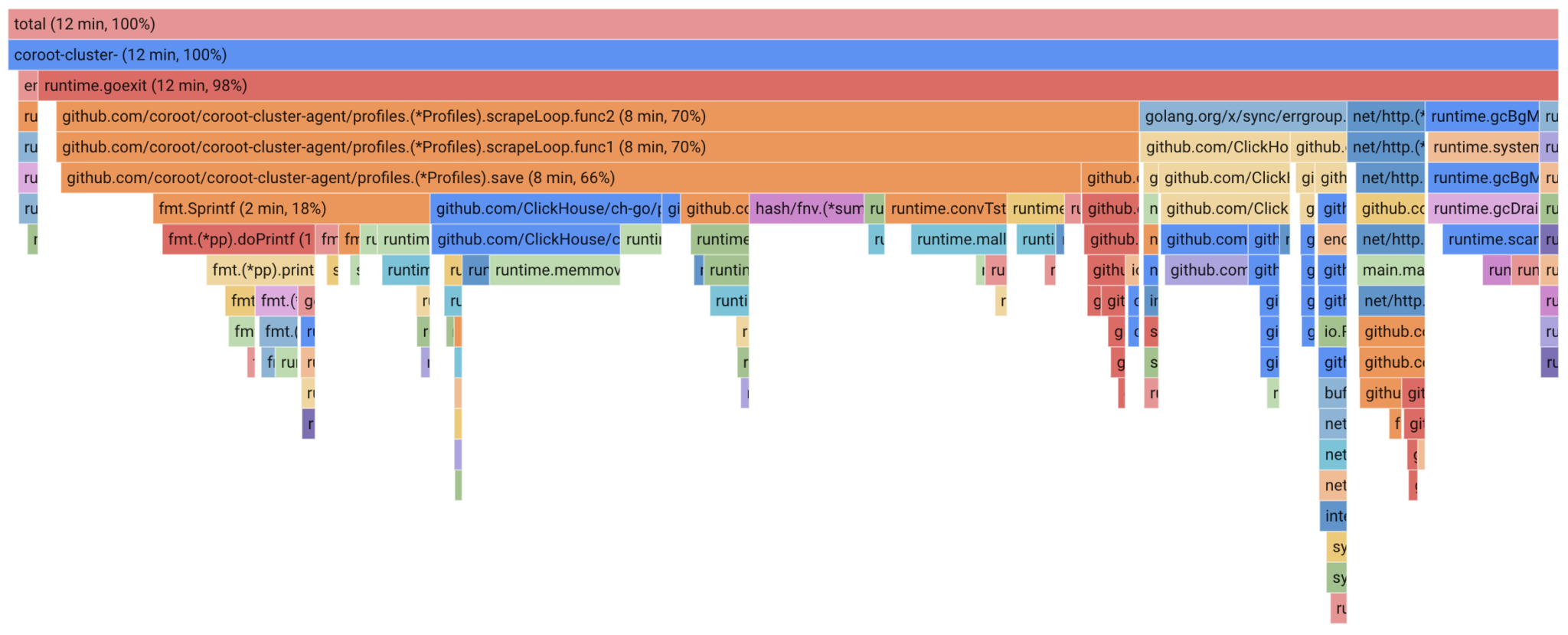
Typically, profiling data is visualized through FlameGraphs. These graphs displays the code hierarchy organized by resource consumption (CPU, Memory). Each frame on the FlameGraph represents the amount of resources consumed by a specific function. A wider frame signifies greater resource consumption by that function, with frames underneath indicating nested function calls.

Profiling data model

Roughly speaking, a profile is a set of measurements, each represented by a value and linked to a corresponding call stack. For example, we observe two call stacks that share two common parts.

Value	Call stack
5 seconds	main→handleRequest→serializeResponse→json.Marshall
10 seconds	main→handleRequest→queryDatabase

The FlameGraph for this profile would look as follows:

The main and handleRequest functions consumed a total of 15 seconds (5 + 10). This consumption was then distributed between queryDatabase and serializeResponse. Examining this FlameGraph makes it clear that queryDatabase consumes twice as much as serializeResponse. Pretty straightforward, isn’t it?

Now, let’s consider profiling our app once a minute. Each measurement should be annotated with the relevant timestamp.

Time	Value	Call stack
60	5 seconds	main→handleRequest→serializeResponse→json.Marshall
60	10 seconds	main→handleRequest→queryDatabase
120	3 seconds	main→handleRequest→serializeResponse→json.Marshall
120	7 seconds	main→handleRequest→queryDatabase

To render the aggregated FlameGraph, we need to sum the values for the same corresponding call stacks.

If we are profiling multiple applications in our cluster, we need a way to distinguish their profiles. Therefore, let’s add labels for each measurement:

Time	Labels	Value	Call stack
60	{ns: default, pod: catalog-xxx-111}	5 seconds	main→handleRequest→serializeResponse→json.Marshall
60	{ns: default, pod: catalog-xxx-111}	10 seconds	main→handleRequest→queryDatabase
60	{ns: default, pod: catalog-xxx-2222}	5 seconds	main→handleRequest→serializeResponse→json.Marshall
60	{ns: default, pod: catalog-xxx-2222}	10 seconds	main→handleRequest→queryDatabase
120	{ns: default, pod: catalog-xxx-1111}	3 seconds	main→handleRequest→serializeResponse→json.Marshall
120	{ns: default, pod: catalog-xxx-1111}	7 seconds	main→handleRequest→queryDatabase
120	{ns: default, pod: catalog-xxx-2222}	3 seconds	main→handleRequest→serializeResponse→json.Marshall
120	{ns: default, pod: catalog-xxx-2222}	7 seconds	main→handleRequest→queryDatabase

Implementing this schema directly in ClickHouse doesn’t seem efficient due to the repetition of potentially long call stacks. Our solution involves storing stacks in a separate table, and values reference them using short hashes.

This approach significantly reduces the amount of data read from disk during queries, as each unique call stack is read only once after aggregating values. As a result, ClickHouse has to decompress less data, leading to lower CPU consumption and improved query latency.

The profiling_samples table stores values along with their corresponding stack hashes (8 bytes per hash):

CREATE TABLE profiling_samples
(
    `ServiceName` LowCardinality(String) CODEC(ZSTD(1)),
    `Type` LowCardinality(String) CODEC(ZSTD(1)),
    `Start` DateTime64(9) CODEC(Delta(8), ZSTD(1)),
    `End` DateTime64(9) CODEC(Delta(8), ZSTD(1)),
    `Labels` Map(LowCardinality(String), String) CODEC(ZSTD(1)),
    `StackHash` UInt64 CODEC(ZSTD(1)),
    `Value` Int64 CODEC(ZSTD(1))
)
ENGINE = MergeTree
PARTITION BY toDate(Start)
ORDER BY (ServiceName, Type, toUnixTimestamp(Start), toUnixTimestamp(End))
TTL toDateTime(Start) + toIntervalDay(7)
SETTINGS index_granularity = 8192

Call stacks are stored in the profiling_stacks table. Since there’s no need to store identical stacks multiple times, we can leverage the ReplacingMergeTree engine, which automatically eliminates repetitions from the table.

CREATE TABLE profiling_stacks
(
    `ServiceName` LowCardinality(String) CODEC(ZSTD(1)),
    `Hash` UInt64 CODEC(ZSTD(1)),
    `LastSeen` DateTime64(9) CODEC(Delta(8), ZSTD(1)),
    `Stack` Array(String) CODEC(ZSTD(1))
)
ENGINE = ReplacingMergeTree
PARTITION BY toDate(LastSeen)
PRIMARY KEY (ServiceName, Hash)
ORDER BY (ServiceName, Hash)
TTL toDateTime(LastSeen) + toIntervalDay(7)
SETTINGS index_granularity = 8192

As you can see, both tables have timestamp-based TTLs, allowing us to configure the duration for which we want to retain profiling data.

Now, let’s examine the compression ratio. Below are statistics from our test environment with a few dozen services over 7 days:

SELECT
    table,
    formatReadableSize(sum(data_compressed_bytes) AS csize) AS compressed,
    formatReadableSize(sum(data_uncompressed_bytes) AS usize) AS uncompressed,
    round(usize / csize, 1) AS compression_ratio,
    sum(rows) AS rows
FROM system.parts
WHERE table LIKE 'profiling_%'
GROUP BY table

Query id: c7edc73e-c225-45ad-81dc-76d623cd078d

┌─table──────────────┬─compressed─┬─uncompressed─┬─compression_ratio─┬──────rows─┐
│ profiling_stacks   │ 931.50 MiB │ 13.68 GiB    │                15 │  16058148 │
│ profiling_samples  │ 6.19 GiB   │ 75.05 GiB    │              12.1 │ 923695809 │
└────────────────────┴────────────┴──────────────┴───────────────────┴───────────┘

As evident, the profiling_stacks table contains 60 times fewer rows than profiling_samples, highlighting the effectiveness of our manual optimization. Additionally, the compression ratios appear to be quite impressive.

Querying profiling data

Using the described schema, we can use the following query to aggregate all measurements for a given service and time interval. This query aggregates measurement values by StackHash and then retrieve the relevant stacks by their hashes.

WITH
    samples AS
    (
        SELECT
            StackHash AS hash,
            sum(Value) AS value
        FROM profiling_samples
        WHERE
            ServiceName IN ['/k8s/default/catalog'] AND
            Type = 'go:profile_cpu:nanoseconds' AND
            Start < toDateTime64('2024-01-25 10:17:15.000000000', 9, 'UTC') AND
            End > toDateTime64('2024-01-25 09:17:15.000000000', 9, 'UTC')
        GROUP BY StackHash
    ),
    stacks AS
    (
        SELECT
            Hash AS hash,
            any(Stack) AS stack
        FROM profiling_stacks
        WHERE
            ServiceName IN ['/k8s/default/catalog'] AND
            LastSeen > toDateTime64('2024-01-25 09:17:15.000000000', 9, 'UTC')
        GROUP BY Hash
    )
SELECT
    value,
    stack
FROM samples
INNER JOIN stacks USING (hash)

...

1454 rows in set. Elapsed: 0.459 sec. Processed 968.75 thousand rows, 66.77 MB (2.11 million rows/s., 145.61 MB/s.)

In the result, we’ve obtained all the necessary data to render a FlameGraph. All aggregation across application instances and profiles is handled on the ClickHouse side, eliminating the need for additional computation on top of this data. The query latency is quite low and does not drastically change for longer time periods, as most of the time is spent on retrieving call stacks, and they are usually the same for any particular app.

Results

Using ClickHouse for storing profiling data has proven to meet all our storage requirements:

Storage efficiency
Configurable data retention
Low latency
Easy to support and maintain
Permissive open-source license

As a bonus, fully integrating ClickHouse as a storage solution for profiling data, along with our custom FlameGraph UI implementation, required less code compared to integrating with Pyroscope.

Try Coroot Cloud now (14-day free trial is available) or follow the instructions on our Getting started page to install Coroot Community Edition.

If you like Coroot, give us a ⭐ on GitHub️.

Any questions or feedback? Reach out to us on Slack.